
A simple yet comprehensive standardized safety stock formula that has proven to be effective in multiple Fortune 500 organizations.
Safety stock. This pesky inventory concept invokes both anxiety and confusion among supply chain professionals, and the debate over the calculation and application of safety stock lives on ruthlessly in a post-COVID world. However, as the current supply chain landscape reels from the effects of an ineffective safety stock model, online research on the topic often results in a plethora of formulas, inconclusive recommendations, and/or questionable logic behind those proposed calculations. In addition, many theories and strategies are discussed, to include: dynamic versus static safety stock; historical usage versus forecasted demand for estimating reserves; accounting for unpredictability, supplier failures, force majeure events, and significant demand fluctuations; and, segregating buffer stock and safety stock versus one lump sum (among other elements). Unfortunately, most resources online only create more questions than provide answers, and this often leaves support seekers feeling worse than when they started their web searches.
If you are interested in learning more about safety stock theory, finding definitive answers to your safety stock questions, and being introduced to a formula developed across ten years of industry learnings in three Fortune 500 companies (all of whom adopted the safety stock formula to great success), please continue to read. By the end of this article, the help you’re seeking will be provided—our promise to you for investing 20 minutes of your time.
A SHORT BACKSTORY
Years back when I was a material planner, I never knew what I was going to walk into the next day… And that was if I was even able to make it to the next day! From calls in the middle of the night to blindsided midday bombardments by leadership, part shortages were an ever present pain point to the role. As a natural problem solver, I desperately wanted to find a way to stop the chaos and uncertainty.
I started by breaking back into my old university textbooks and searching online for answers. It was clear a better application of inventory protection was needed, but safety stock formulas were “a dime a dozen” all over the internet. There must have been a hundred of them I reviewed, and they all claimed to solve the safety stock conundrum; but, it became obvious these formulas were created by people who 1) never sat in the planning role, 2) had not seen the day to day planning environment in years, and/or 3) failed to provide the logic behind their calculations.
My frustration led me back to my mathematical roots, and I landed on the theoretical concepts of estimation. In a seemingly unrelated exercise, I was attempting to budget for my personal finances using finite and infinite population sampling, point and interval estimates, and even creating upper and lower limits in spectacularly nerdy fashion when it dawned on me: there is a read across to inventory levels here! I began formulating a safety stock equation that has now been tested, refined, and proven through a decade of industry ups and downs to include a recession and a pandemic.
The goal I was trying to achieve was to logically apply sound math to the real world. I love the quote, “If the math is right, we cannot fail.” When it comes to inventory and planning, there is no truer statement. What I learned most during my time in Corporate America was that inventories were rarely “right-sized.” Companies always seemed to have too much of what they didn’t need and not enough of what they did. We have all seen this walking through the grocery store from time to time, let alone within the company we work for, I bet. However, to get to the optimal, right-sized safety stock equation, I needed to educate myself on several key topics concerning safety stock, trial and error multiple methodologies, and conclusively land on the right-fit formula for a right-sized inventory.
Disclaimer: We recognize there are a multitude of talking points on safety stock theory and application, more than we can effectively cover in this article, but we also do not want to get caught up and/or distracted with safety stock concepts that do not add the most value to this conversation. With that said, let’s go ahead and rapid fire through the leading topics below.

Dynamic Versus Static Safety Stock
Without a doubt, a dynamic safety stock should be used when possible. If you have features in your MRP system such as coverage profile or automated inventory reserves, those are the ideal states in our opinion. However, the systems still have to be told what period of time or days of coverage should be entered, so a competent safety stock formula and process are required.
On the static front, if your company has chosen to implement this type of a model for safety stock, or your current MRP system only offers a static quantity field for reserves, do not fret. In either situation, dynamic or static, the safety stock formula below is a great fit.
Safety Stock Update Timing
This is always an interesting debate, and every large Fortune 500 company we have worked for selected a different cadence for refreshing the numbers and updating the system. Although program or part life cycle and company-specific seasonality play a role in picking the optimal update period, if you need to start somewhere, we would recommend a monthly update. You may find this might be too frequent and wastes administrative resources, but we would not advise on updating less frequent than quarterly. However, if you have certain parts phasing in or out, those probably need to be classified or categorized separately with a more frequent update cadence (two weeks to one month).
Historical Usage Versus Forecasted Demand for Estimating Reserves
Both need to be used; they each provide a critical piece to the safety stock formula.
Accounting for Unpredictability, Supplier Failures, Force Majeure Events, and Significant Demand Fluctuations
This is a must, and it also has to make quantifiable sense.
Segregating Buffer Stock and Safety Stock Versus One Lump Sum
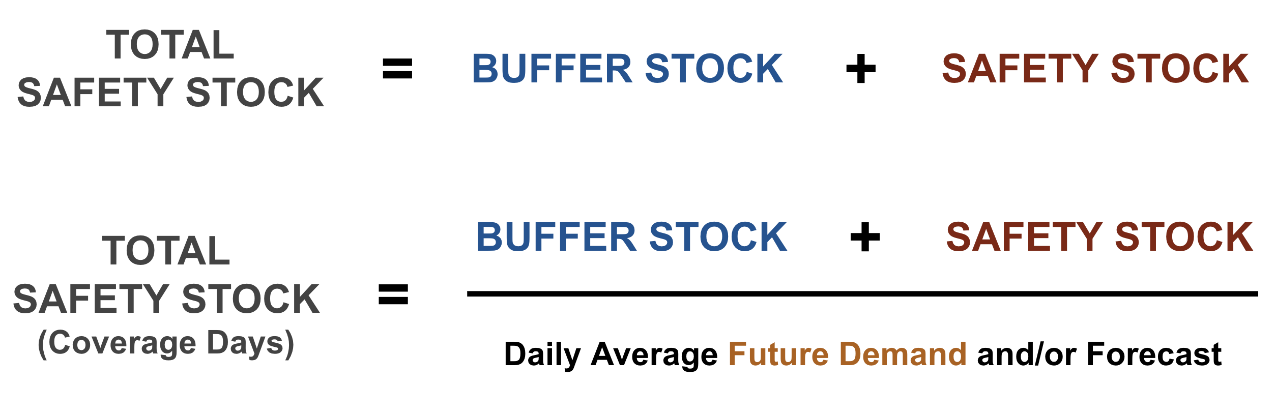
Buffer stock and safety stock protect for two different things, and it is crucial to understand the difference between them. Buffer stock covers for common cause variance between deliveries to include a short term demand spike, a scrap or inventory adjustment event, or a shipment delivering a day late. Safety stock protects for special cause variance for full supplier lead time such as long term demand increases, an unreliable supplier, a force majeure event, or a port strike. By adding these two together, we get a total safety stock which offers comprehensive protection.
The irony behind this debate is that the same outcome is desired by adopters in both camps. Those who segregate and calculate buffer and safety stock individually usually end up adding them back together for one lump sum while others who calculate for one lump sum are hoping to protect for both common cause and special cause variances. Regardless of your preference, the safety stock formula provided below supports both models.

Now, let’s dig into the formulas and sub-elements used to calculate buffer stock and safety stock, why these elements are included, and the mathematical principles applied to each one within the formulas.
BUFFER STOCK FORMULA
For the exact buffer stock tabular software calculation for Microsoft Excel or Google Sheets, please message us for a free tutorial and sample Microsoft Excel file that will walk through the data and calculation step-by-step.

Historical Consumption
Based on the estimation concepts of finite sampling and point estimation, use the standard deviation of historical consumption (to include scrap and inventory adjustments with outliers removed) over a period of time. This length of time is usually 3, 6, or 12 months; the default can be 6 months, but this is usually determined by the stability and/or maturity of the part number. More time is needed if the part is experiencing dramatic fluctuations in consumption (we are looking at you, COVID-19 impact), while less time if the part is phasing in or out (3 months or less).
Standard deviation of historical consumption is the best indicator we have found to predict short term variance because it is based on what actually occurred with the part during a period of time. The logic here is that the past often proves the future for common cause variance.
Important Note: When calculating for the standard deviation of historical consumption, it is imperative to use total days instead of working days. In other words, include all 7 days of the week, even if your company does not consume on certain days. For example, if you have selected a 90 day period of time for historical consumption, calculate the standard deviation for all 90 days (even if some days have no consumption). This is important when aligning with the replenishment frequency.
Replenishment Frequency
Replenishment frequency is calculated by counting the days between deliveries for a part number. In other words, if a part is delivered from a supplier every week on Monday, then the replenishment frequency would be 7. If the part is delivered twice a week, then the replenishment frequency would be 3.5 (7/2). If the part is internationally sourced and delivers monthly, then the replenishment frequency would be 30.
Important Note: Replenishment frequency is always calculated based on a seven day week.
Service Level
Service level is the level of service and support a company wants to provide its customers, and it is subjective. Typically, we have seen this used as a very low, low, medium, high, and very high type of setup, with 85% (very low), 90% (low), 95% (medium), 97% (high), and 99% (very high) being utilized in the formula. In layman’s terms, service level is the percent of a customer’s common cause variance a company would like to protect for. A good starting point is 95%, but organizational leadership usually sets the service level.
Important Note: When utilizing service level within the buffer stock calculation, the inverse of the standard normal cumulative distribution of service level will be used (in Microsoft Excel and Google Sheets, this is the “NORMSINV” function). More specifically, “NORMSINV” provides a value for a cumulative probability using a standard normal distribution. Since the assumption is that the data is normally distributed, use this function to know the value for the probability of service level.
SAFETY STOCK FORMULA
Again, for the exact safety stock tabular software calculation for Microsoft Excel or Google Sheets, please message us for a free tutorial and sample Microsoft Excel file that will walk through the data and calculation step-by-step.

Future Demand
Based on the estimation concepts of infinite sampling and point estimation, use the daily average of future demand and/or forecast over a period of time. This length of time is usually 3, 6, or 12 months; the default can be 6 months, but this is usually determined by the stability and/or maturity of the part number. Less time is needed if the part is experiencing dramatic fluctuations in demand or if the part is phasing in or out (the opposite of the historical consumption time recommendations).
Important Note: The daily average of future demand and/or forecast should be based on working days, not total days (unless consumption occurs every day). In other words, if the next 3 months of forecast (90 days) is 20,000 units, and the company only consumes Monday through Friday, then divide the 20,000 by 64 working days (estimated working days from the 90) instead of 90. The logic here is that the safety stock needs to offer “apples to apples” protection for how and in what quantities an organization consumes the part.
Risk Level
Risk level is the level of risk attached to a part. Typically, we have seen this used as a very low, low, medium, high, and very high type of setup, with 5% (very low), 12% (low), 20% (medium), 25% (high), and 30% (very high) being utilized in the formula. A good starting point is 12%, and planners usually choose the risk level based on their experience with managing the part. For example, if you are a planner managing a part from an unreliable supplier, it may be apparent that one in five orders is delivered late. Since this is not a “one-off” situation and the supplier is habitually offending with late deliveries, it would be prudent to select a 20% risk level (one late delivery divided by the five total). On the contrary, if you have a reputable supplier who always delivers on time and/or is right down the road in the same town as my company, you may drop the risk level to 5%. Similar to service level for buffer stock, risk level is the subjective element to the safety stock formula, and it needs to be controlled by the person closest to the part.
Supplier Lead Time
Supplier lead time refers to the full, “cold start” lead time a supplier is contracted to (this is not the same as trade off zone or the raw materials buyout period). Special cause variance can include scenarios that might bring the supplier back to cold start lead times to support the request or resolve the issue, so that is why it is used for the safety stock formula. However, utilize only the square root of supplier lead time in the formula, and this was something tweaked a few years ago to support Lean inventory initiatives. It still provides adequate protection, but eliminates the surplus on long lead time parts.
TOTAL SAFETY STOCK FORMULA
LET’S CONNECT
We hope you enjoyed the article and found it informative and helpful. We are confident it will work for you and your company even if it requires some minor tweaking. All organizations are unique, but the beauty in process knowledge and best practice sharing is that they can either be used “as-is” or as the foundation for more custom, tailored-fit solutions.
We understand readers are curious about the inventory and expedited shipment reductions achieved when using this formula based on the comments and questions already received. It is critical to have sound material planning processes in place to support many other issues the role faces (another article is coming soon on this topic from the Perfect Planner Team), but typically a 15-35% reduction in inventory and 50-80% reduction in expedited shipments are common after implementing the total safety stock formula. The timing to see these results varies based on your company’s supplier lead times which dictate how quickly existing safety stocks can be increased or decreased. It’s worth the wait, though, as these results are what we personally witnessed at several Fortune 500 companies, and they are also why we are assured in sharing the safety stock formula with you.
If you have questions or would like to see if the formula can be reworked to accommodate your specific business practices, please reach out. The Perfect Planner Team offers a free consultation service, and we are here to serve. We also highly recommend messaging us to request the sample Microsoft Excel file and video tutorial taking you step-by-step through the calculation with data. These are free resources–by planners, for planners–to help you on your journey.
We would also love to hear from you! The Perfect Planner Team desires to create content that supports the people doing the jobs and the leaders managing those jobs. If there is a particular topic in supply chain or operations you would like us to cover, please message us and request it.
Happy planning!
Author: Thomas Beil
Publication Date: October 2, 2022
© Copyright 2023 Perfect Planner LLC. All rights reserved.